*** This tutorial requires backgound on general controls. ***
Introduction
This tutorial will cover applying different controls to motors - especially brushless motors. I would like to point out there is an excellent series of video presentations from Texas Instruments on how to control motors. This tutorial will cover the same topics, but in a written way rather than in video format. This tutorial is meant to be a fast way to look up derivations for various controller designs.
https://www.youtube.com/watch?v=cdiZUszYLiA - Field oriented control of permanent magnet motors
https://www.youtube.com/watch?v=fpTvZlnrsP0 - Teaching old motors new tricks (part 1 of 5)
Current Control
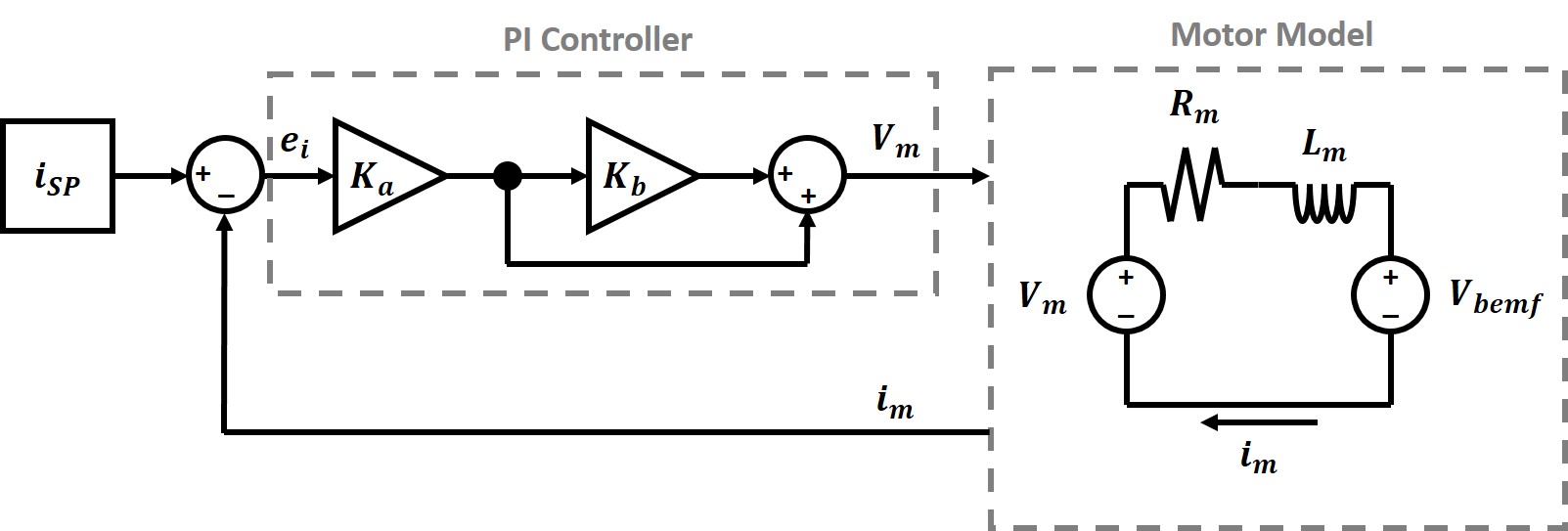
Figure 1. Block diagram for a cascaded PI controller. Output from the PI controller is voltage powering the motor, while feedback is the current measured from the motor coil.
A current controller can be a simple PI controller (no derivative term needed). There are different ways to implement a PI controller, but for motor control it is easier to calculate the coefficients when using a cascaded controller (Fig. 1.) The two gain coefficients are \(K_a\) and \(K_b\). Compared to a more standard PI controller \(K_p = K_a\) and \(K_i = K_a K_b\). Going through the full closed loop controller gain will show why the cascaded form of PI controller is preferable. First we will start with the transfer function for the PI controller and the transfer function for the motor. \[ \frac{V_m (S)}{e_i (S)} = \frac{S K_a + K_a K_b}{S} \tag{1} \] \[\frac{i_m(S)}{V_m(S)} = \frac{J_m S}{K_m^2+(R_m J_m)S + (L_m J_m)S^2} \tag{2} \] \(e_i\) is the current error (the difference between the setpoint current and the measured current). One thing we assume in this analysis is that the motor inertia is large, so the rate of change of current in the motor is much faster than the rate of change in velocity of the motor. This simplifies the motor circuit transfer function to an L R cirucit. \[ \frac{i_m (S)}{V_m (S)} = \frac{1}{R_m + L_m S} \tag{3} \] The open loop gain can be calculated by cascading the PI controller and motor transfer functions. \[ G_{OL}(S)=\frac{i_m (S)}{e_i (S)} = \frac{K_a K_b + K_a S}{S(R_m + L_m S)} \tag{4} \] The closed loop gain can be derived from the open loop gain. \[ G_{CL}(S) = \frac{G_{OL}(S)}{1+G_{OL}(S)} = \frac{i_m(S)}{i_{SP}(S)} = \frac{K_a (K_b + S)}{K_a K_b + (K_a + R_m)S + L_m S^2} \tag{5} \] Now lets figure out the optimal values for \(K_a\) and \(K_b\). First, lets look at the poles of \(G_{CL}(S)\). \[ S = \frac{-(K_a + R_m) \pm \sqrt{(K_a + R_m)^2 - 4 K_a K_b L_m} }{2 L_m} \tag{6} \] Let's try setting \(K_b = R_m / L_m\) and looking at the poles of \(G_{CL}(S)\). \[ S = \frac{-(K_a + R_m) \pm \sqrt{(K_a + R_m)^2 - 4 K_a R_m} }{2 L_m} \tag{7} \] \[ S = \frac{-(K_a + R_m) \pm \sqrt{K_a ^2 - 2 K_a R_m + R_m ^2} }{2 L_m} \tag{8} \] \[ S = \frac{-(K_a + R_m) \pm \sqrt{(K_a - R_m)^2} }{2 L_m} \tag{9} \] \[ S = \frac{-(K_a + R_m) \pm (K_a - R_m) }{2 L_m} \tag{10} \] \[ S = \frac{-K_a }{L_m} , \frac{-R_m}{L_m} \tag{11} \] Now we can look at the zero when \(K_b = R_m / L_m\). \[ S = - \frac{R_m}{L_m} \tag{12} \] It can be seen that the zero cancels out one of the poles, so the final transfer function becomes a first order system. \[ G_{CL}(S) = \frac{K_a(\frac{R_m}{L_m}+S)}{(K_a + L_m S)(\frac{R_m}{L_m}+S)} = \frac{1}{1 + \frac{L_m}{K_a} S}\tag{13} \] In this final form it can be seen that the bandwidth of the system is \(K_a / L_m\). To summarize, a cascaded PI controller should have the following gains: \[K_a = L_m * Current Bandwidth \] \[K_b = \frac{R_m}{L_m} \]