*** This tutorial requires some background on differential equations and laplace transforms. ***
Introduction
This tutorial will cover how to make a mathematical model for an electric motor - an essential part of developing a control system for an electric motor. An electric motor is anything that creates mechanical motion from an electrical input. The majority use magnetic fields to generate the forces needed for motion. Motion is not limited to rotation and can also include linear motion. For this tutorial we will be working on a basic model for a magnetic electric motor. Modeling can start with separate electrical and mechanical models and later combined to form a complete electro-mechanical model of the system.
Electrical Model
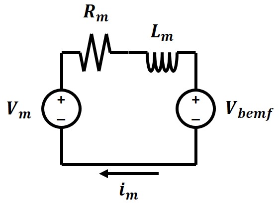
Figure 1. Electrical model of a generic electric motor. Voltage is set as the input since motor controllers typically output a voltage.
Let's start with the electrical portion of a motor. An electric motor can be drawn as a simplified circuit containing two voltage supplies, an inductor, and a resistor (Fig. 1). The first voltage source labeled as \(V_m\) is the input voltage from an external source. This external soruce could be a battery, power supply, motor controller, or even another motor. The inductor and resistor labeled as \(L_m\) and \(R_m\) model the electromagnetic coils in the motor. The second voltage source labeled as \(V_bemf\) represents the voltage generated by the motor when spinning. All motors can function as generators. A voltage is generated on a coil of wire when a coil of wire is subject to a changing magnetic field (the magnet in a motor sweeping by the coil). For now we can write an equation that relates the input voltage \(V_m\) to the current in the coil \(i_m\), but we will need to expand out the \(V_{bemf}\) term to model the motion of the motor. \[V_m = R_m i_m + L_m \dot{i_m} + V_{bemf} \tag{1}\]
Mechanical Model
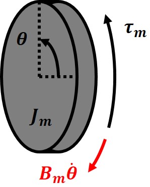
Figure 2. Mechanical model of a generic rotary electric motor. An input torque can accelerate or decelerate the rotational mass of the motor.
The mechanical model of the motor can be drawn as a rotating mass with an applied torque (Fig. 2). The rotational inertia of the motor is \(J_m\), while the input torque is \(\tau_m\). An additional damping term \(B_m\) is included to account for friction. This term simulates viscous damping that is proportional to rotational velocity, rather than friction which may be constant or non-linear. The equation of motion for the motor relates input torque to angular acceleration \(\ddot{\theta}\). \[\tau_m = J_m \ddot{\theta} + B_m \dot{\theta} \tag{2}\] Notice that angle (\(\theta\)) does not appear in the equation of motion. Torque on the motor will create acceleration (\(\ddot{\theta}\)), so the position is irrelevant for this model.
Electrical to Mechanical Relationship
We need a relationship to combine the electrical and mechanical models and determine \(V_{bemf}\) and \(\tau_m\). This relationship is the motor's KV. KV is a common specification for a motor and relates the rotational speed of the motor to the input voltage. An example motor might have a KV of 350, which means the motor will spin at 350 RPM with 1V applied. For the model we will convert KV to units of volts per radian per second and call this constant \(K_{m}\). \(V_{bemf}\) can now be related to the mechanical model. \[V_{bemf} = K_{m} \dot{\theta} \tag{3} \] Motor torque is proportional to coil current. Interestingly the speed constant of the motor, \(K_m\), is also the torque constant of the motor. The torque constant has units of newton meters per amp. If the units of both the speed constant and torque constant are reduced to the most basic units, they both become \(m^2 {kg} /{s^2 A}\). \(\tau_m\) can now be related to the electrical model. \[\tau_m = K_{m} i_m \tag{4} \]
Complete Motor Model
The complete motor model is summarized with two equations covering the mechanical and electrical domains \[V_m = R_m i_m + L_m \dot{i_m} + K_{m} \dot{\theta} \tag{5}\] \[K_{m} i_m = J_m \ddot{\theta} + B_m \dot{\theta} \tag{6}\] A few important parameters can be observed by looking at edge cases of these equations in the steady state. The first edge case is when \(V_{bemf} = K_m \dot{\theta} = V_m \). This is the *fastest* the motor can rotate with the applied \(V_m\) and is also called the free speed of a motor. Note that no current can be flowing in the motor. In a real motor there will always need to be some current flowing to provide the torque necessary to overcome various sources of friction. The second edge case is when the motor is not rotating \(\dot{\theta} = 0\). This is the *highest* current a motor can draw and is called the stall current of a motor. Along with stall current comes stall torque, which is the torque generated when the motor is stalled. this is also the *highest* torque a motor can output. I put asterisks around these parameters since there are conditions where these values can be exceeded. One example is if a motor is spinning backwards and a full forward voltage is applied. Now \(V_{bemf}\) and \(V_m\) add together such that the motor coils see a significantly higher voltage. This in turn can generate double the stall current and torque.
Motor Dynamics
Now we can look at the dynamics of the system. To simplify the analysis we will take the laplace transforms of both the electrical and mechanical equations. \[K_m i_m(S) = J_m \theta(S)S^2 + B_m \theta(S)S \tag{7} \] \[V_m(S) = R_m i_m(S) + L_m i_m(S)s + K_m \theta(S)S \tag{8}\] Now depending on what response we want we can rearrange to find a transfer function. The transfer function will relate an input to an output. In the case of the motor model, it is important to see the response of position and current from an input voltage. \[\frac{\theta(S)}{V_m(S)} = \frac{K_m}{S((R_m B_m + K_m^2)+(R_m J_m + B_m L_m)S +(L_m J_m)S^2)} \tag{9} \] \[\frac{i_m(S)}{V_m(S)} = \frac{B_m + J_m S}{(K_m^2 + R_m B_m)+(R_m J_m + L_m B_m)S + (L_m J_m)S^2} \tag{10} \] Additionally we can derive the response of position from an input of current. \[\frac{\theta(S)}{i_m(S)} = \frac{K_m}{S(B_m + J_m S)} \tag{11} \] An interesting comparison can be seen in the difference between the position response to an input voltage and an input current to the motor. The position response can be converted to an angular velocity response by taking the derivative, or multiplying the transfer function by S. In the absence of damping \(B_m = 0\), both (9) and (11) can be rewritten to show the response of angular velocity \(\omega\). \[\frac{\omega(S)}{V_m(S)} = \frac{K_m}{K_m^2+(R_m J_m)S +(L_m J_m)S^2 } \tag{12} \] \[\frac{\omega(S)}{i_m(S)} = \frac{K_m}{J_m S} \tag{13} \] Controlling a motor with voltage gives the motor an inherent damping term. intuitively, \(V_{bemf}\) causes damping since it reduces the effective voltage over the coil as the motor speeds up. Voltage is needed to drive the current in the coil, which in turn creates the torque. In the motor control tutorial it can be seen it is easier to use high gains on a voltage controlled motor due to this additional damping term.